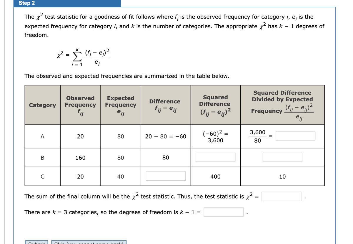
Step 2 The x test statistic for a goodness of fit follows where f; is the observed frequency for category i, e; expected frequency for category i, and k is the number of categories. The appropriate x...


Step 2<br>The x test statistic for a goodness of fit follows where f; is the observed frequency for category i, e;<br>expected frequency for category i, and k is the number of categories. The appropriate x has k<br>is the<br>1 degrees of<br>freedom.<br>k<br>= (f, - e)?<br>i = 1<br>The observed and expected frequencies are summarized in the table below.<br>Expected<br>Frequency<br>Squared<br>Difference<br>Squared Difference<br>Divided by Expected<br>Observed<br>Difference<br>Category<br>Frequency<br>(fj – e;)²<br>eij<br>fij - eij<br>(fj – @j)²<br>fj<br>eij<br>Frequency<br>(-60)2<br>3,600<br>3,600<br>A<br>20<br>80<br>20<br>80 = -60<br>%D<br>80<br>В<br>160<br>80<br>80<br>20<br>40<br>400<br>10<br>The sum of the final column will be the x test statistic. Thus, the test statistic is x<br>=<br>There are k<br>= 3 categories, so the degrees of freedom is k – 1 =<br>Cubri4<br>Cli<br>

Extracted text: Step 2 The x test statistic for a goodness of fit follows where f; is the observed frequency for category i, e; expected frequency for category i, and k is the number of categories. The appropriate x has k is the 1 degrees of freedom. k = (f, - e)? i = 1 The observed and expected frequencies are summarized in the table below. Expected Frequency Squared Difference Squared Difference Divided by Expected Observed Difference Category Frequency (fj – e;)² eij fij - eij (fj – @j)² fj eij Frequency (-60)2 3,600 3,600 A 20 80 20 80 = -60 %D 80 В 160 80 80 20 40 400 10 The sum of the final column will be the x test statistic. Thus, the test statistic is x = There are k = 3 categories, so the degrees of freedom is k – 1 = Cubri4 Cli
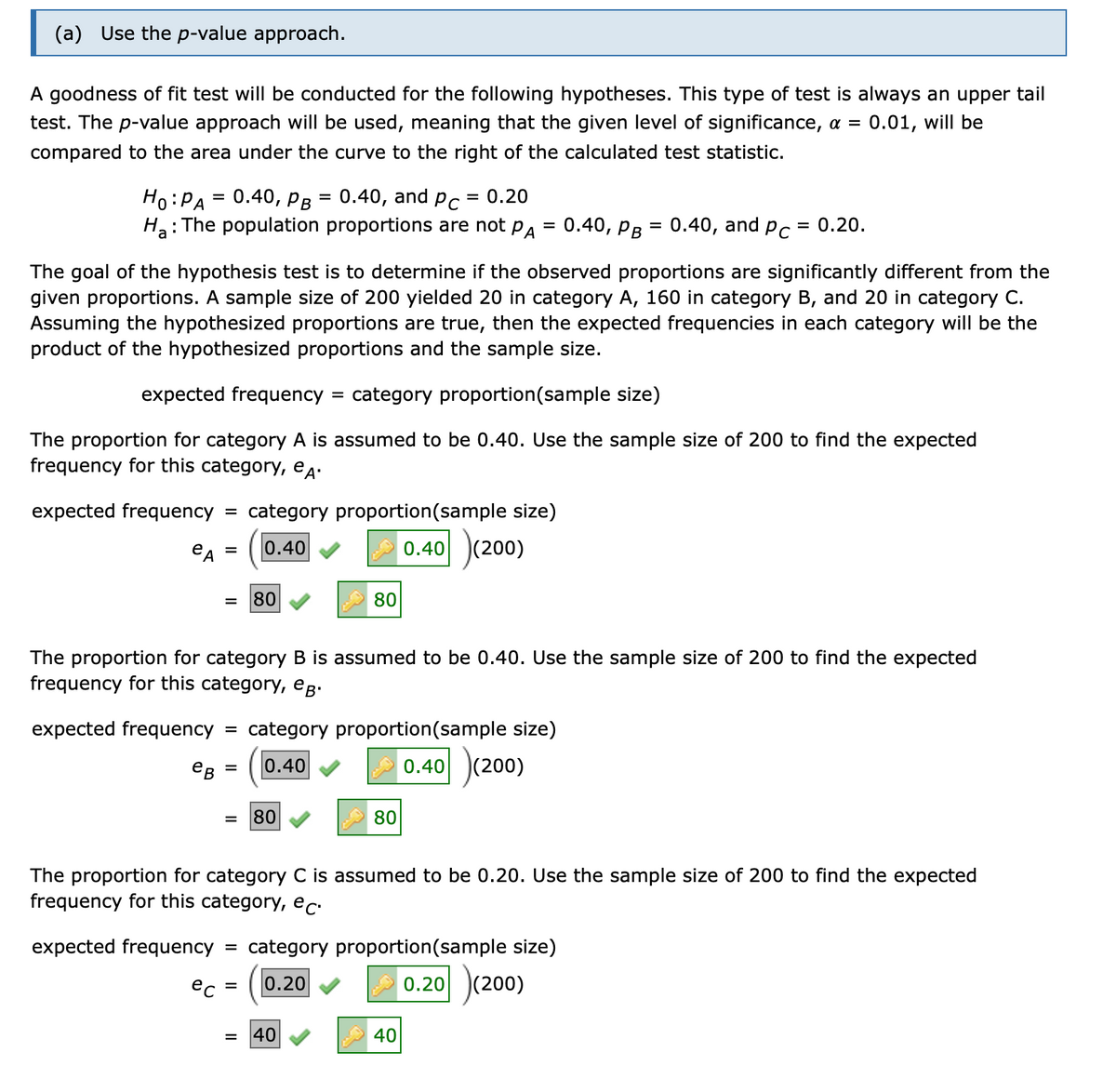
(a) Use the p-value approach.<br>A goodness of fit test will be conducted for the following hypotheses. This type of test is always an upper tail<br>test. The p-value approach will be used, meaning that the given level of significance, a =<br>0.01, will be<br>compared to the area under the curve to the right of the calculated test statistic.<br>0.40, PB = 0.40, and<br>= 0.20<br>Ho:PA<br>H: The population proportions are not pa = 0.40, pB = 0.40, and pc<br>Pc<br>= 0.20.<br>The goal of the hypothesis test is to determine if the observed proportions are significantly different from the<br>given proportions. A sample size of 200 yielded 20 in category A, 160 in category B, and 20 in category C.<br>Assuming the hypothesized proportions are true, then the expected frequencies in each category will be the<br>product of the hypothesized proportions and the sample size.<br>expected frequency = category proportion(sample size)<br>The proportion for category A is assumed to be 0.40. Use the sample size of 200 to find the expected<br>frequency for this category, ea•<br>expected frequency<br>category proportion(sample size)<br>%D<br>CA =<br>0.40<br>0.40 (200)<br>80<br>80<br>The proportion for category B is assumed to be 0.40. Use the sample size of 200 to find the expected<br>frequency for this category, eg.<br>expected frequency<br>category proportion(sample size)<br>eB =<br>0.40<br>0.40 (200)<br>80<br>80<br>The proportion for category C is assumed to be 0.20. Use the sample size of 200 to find the expected<br>frequency for this category, ec:<br>expected frequency<br>category proportion(sample size)<br>%D<br>ec = (0.20<br>0.20<br>)(200)<br>40<br>40<br>

Extracted text: (a) Use the p-value approach. A goodness of fit test will be conducted for the following hypotheses. This type of test is always an upper tail test. The p-value approach will be used, meaning that the given level of significance, a = 0.01, will be compared to the area under the curve to the right of the calculated test statistic. 0.40, PB = 0.40, and = 0.20 Ho:PA H: The population proportions are not pa = 0.40, pB = 0.40, and pc Pc = 0.20. The goal of the hypothesis test is to determine if the observed proportions are significantly different from the given proportions. A sample size of 200 yielded 20 in category A, 160 in category B, and 20 in category C. Assuming the hypothesized proportions are true, then the expected frequencies in each category will be the product of the hypothesized proportions and the sample size. expected frequency = category proportion(sample size) The proportion for category A is assumed to be 0.40. Use the sample size of 200 to find the expected frequency for this category, ea• expected frequency category proportion(sample size) %D CA = 0.40 0.40 (200) 80 80 The proportion for category B is assumed to be 0.40. Use the sample size of 200 to find the expected frequency for this category, eg. expected frequency category proportion(sample size) eB = 0.40 0.40 (200) 80 80 The proportion for category C is assumed to be 0.20. Use the sample size of 200 to find the expected frequency for this category, ec: expected frequency category proportion(sample size) %D ec = (0.20 0.20 )(200) 40 40
Jun 04, 2022
SOLUTION.PDF

Get Answer To This Question

Related Questions & Answers

More Questions »

Submit New Assignment

Copy and Paste Your Assignment Here