Overview
This project explores gradient-domain processing, a simple technique with a broad set of applications including blending, tone-mapping, and non-photorealistic rendering. For the core project, we will focus on "Poisson blending"; tone-mapping and NPR can be investigated as bells and whistles.
The primary goal of this assignment is to seamlessly blend an object or texture from a source image into a target image. The simplest method would be to just copy and paste the pixels from one image directly into the other. Unfortunately, this will create very noticeable seams, even if the backgrounds are well-matched. How can we get rid of these seams without doing too much perceptual damage to the source region?
The insight is that people often care much more about the gradient of an image than the overall intensity. So we can set up the problem as finding values for the target pixels that maximally preserve the gradient of the source region without changing any of the background pixels. Note that we are making a deliberate decision here to ignore the overall intensity! So a green hat could turn red, but it will still look like a hat.
We can formulate our objective as a least squares problem. Given the pixel intensities of the source image "s" and of the target image "t", we want to solve for new intensity values "v" within the source region "S":

Here, each "i" is a pixel in the source region "S", and each "j" is a 4-neighbor of "i". Each summation guides the gradient values to match those of the source region. In the first summation, the gradient is over two variable pixels; in the second, one pixel is variable and one is in the fixed target region.
The method presented above is called "Poisson blending". Check out thePerez et al. 2003 paperto see sample results, or to wallow in extraneous math. This is just one example of a more general set of gradient-domain processing techniques. The general idea is to create an image by solving for specified pixel intensities and gradients.
Toy Problem (20 pts)
 The implementation for gradient domain processing is not complicated, but it is easy to make a mistake, so let's start with a toy example. Reconstruct this image from its gradient values, plus one pixel intensity. Denote the intensity of the source image at (x, y) as s(x,y) and the value to solve for as v(x,y). For each pixel, then, we have two objectives:
1. minimize (v(x+1,y)-v(x,y) - (s(x+1,y)-s(x,y)))^2
2. minimize (v(x,y+1)-v(x,y) - (s(x,y+1)-s(x,y)))^2
Note that these could be solved while adding any constant value tov, so we will add one more objective:
3. minimize (v(0,0)-s(0,0))^2
For 20 points, solve this in Python as a least squares problem. If your solution is correct, you should recover the original image.
Implementation Details
The first step is to write the objective function as a set of least squares constraints in the standard matrix form: (Av-b)^2. Here, "A" is a sparse matrix, "v" are the variables to be solved, and "b" is a known vector. Especially for blending with irregular masks, it is helpful to keep a matrixim2varthat maps each pixel to a variable number, such as:
im_h, im_w = im.shape
im2var = np.arange(im_h * im_w).reshape(im_h, im_w)
Then, you can write objective 1 above as:
e = e + 1;
A[e][im2var[y][x+1]] = 1
A[e][im2var[y][x]] = -1
b[e] = im[y][x+1] - im[y][x]
Here, "e" is used as an equation counter. Note that the y-coordinate is the first index. As another example, objective 3 above can be written as:
e = e + 1;
A[e][im2var[0][0]] = 1
b[e] = s[0][0]
To solve forv, use
v = scipy.sparse.linalg.lsqr(A, b);
Then, copy each solved value to the appropriate pixel in the output image.
Poisson Blending (50 pts)
Step 1: Select source and target regions. Select the boundaries of a region in the source image and specify a location in the target image where it should be blended. Then, transform (e.g., translate) the source image so that indices of pixels in the source and target regions correspond. The providedutils.pyincludes functions for this. You may want to augment the code to allow rotation or resizing into the target region. You can be a bit sloppy about selecting the source region -- just make sure that the entire object is contained. Ideally, the background of the object in the source region and the surrounding area of the target region will be of similar color.
Step 2: Solve the blending constraints:

Step 3: Copy the solves values into your target image. For RGB images, process each channel separately.
Mixed Gradients (20 pts)
Follow the same steps as Poisson blending, but use the gradient in source or target with the larger magnitude as the guide, rather than the source gradient:

Here "d_ij" is the value of the gradient from the source or the target image with larger magnitude. Note that larger magnitude is not the same as greater value. For example, if the two gradients are -0.6 and 0.4, you want to keep the gradient of -0.6. Show at least one result of blending using mixed gradients. One possibility is to blend a picture of writing on a plain background onto another image.
Bells & Whistles (Extra Points)
Color2Gray (20 pts)
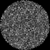
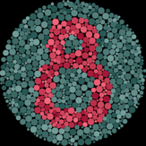
Sometimes, in converting a color image to grayscale (e.g., when printing to a laser printer), we lose the important contrast information, making the image difficult to understand. For example, compare the color version of the image on right with its grayscale version produced by rgb2gray.

Can you do better than rgb2gray? Gradient-domain processing provides one avenue: create a gray image that has similar intensity to the rgb2gray output but has similar gradients to the original RGB image. This is an example of a tone-mapping problem, conceptually similar to that of converting HDR images to RGB displays. For your solution, use only the RGB space (e.g., don't convert to Lab or HSV). Test your solution on colorBlind8.png and colorBlind4.png, included with the sample images. Hint: your solution may be a combination of the toy problem and mixed gradients.
Laplacian pyramid blending (20 pts)
Another technique for blending is to decompose the source and target images using a laplacian pyramid and to combine using alpha mattes. For the low frequencies, there should be a slow transition in the alpha matte from 0 to 1; for the high frequencies, the transition should be sharp. Try this method on some of your earlier results and compare to the Poisson blending.
More gradient domain processing (up to 20 pts)
Many other applications are possible, including non-photorealistic rendering, edge enhancement, and texture or color transfer. SeePerez et al. 2003orGradient Shopfor further ideas.