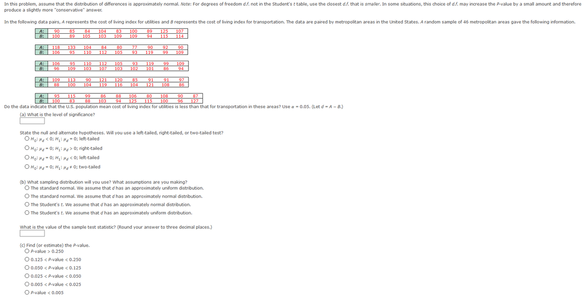
In this problem, assume that the distribution of differences is approximately normal.
Note: For degrees of freedom
d.f. not in the Student's
t
table, use the closest
d.f. that is
smaller. In some situations, this choice of
d.f. may increase the
P-value by a small amount and therefore produce a slightly more "conservative" answer.
In the following data pairs,
A
represents the cost of living index for utilities and
B
represents the cost of living index for transportation. The data are paired by metropolitan areas in the United States.
A
random sample of 46 metropolitan areas gave the following information.

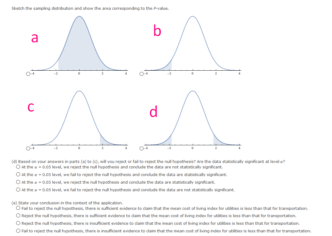
Extracted text: Sketch the sampling distribution and show the area corresponding to the P-value. b a O-4 O-4 -2 C d O-4 O-4 (d) Based on your answers in parts (a) to (c), will you reject or fail to reject the null hypothesis? Are the data statistically significant at level a? O At the a = 0.05 level, we reject the null hypothesis and conclude the data are not statistically significant. O At the a = 0.05 level, we fail to reject the null hypothesis and conclude the data are statistically significant. O At the a = 0.05 level, we reject the null hypothesis and conclude the data are statistically significant. O At the a = 0.05 level, we fail to reject the null hypothesis and conclude the data are not statistically significant. (e) State your conclusion in the context of the application. O Fail to reject the null hypothesis, there is sufficient evidence to claim that the mean cost of living index for utilities is less than that for transportation. O Reject the null hypothesis, there is sufficient evidence to claim that the mean cost of living index for utilities is less than that for transportation. O Reject the null hypothesis, there is insufficient evidence to claim that the mean cost of living index for utilities is less than that for transportation. O Fail to reject the null hypothesis, there is insufficient evidence to claim that the mean cost of living index for utilities is less than that for transportation.

0; right-tailed O Ho: Hd = 0; H;: Hd < 0;="" left-tailed="" o="" ho:="" hd="0;" h:="" hd#="" 0;="" two-tailed="" (b)="" what="" sampling="" distribution="" will="" you="" use?="" what="" assumptions="" are="" you="" making?="" o="" the="" standard="" normal.="" we="" assume="" that="" d="" has="" an="" approximately="" uniform="" distribution.="" o="" the="" standard="" normal.="" we="" assume="" that="" d="" has="" an="" approximately="" normal="" distribution.="" o="" the="" student's="" t.="" we="" assume="" that="" d="" has="" an="" approximately="" normal="" distribution.="" o="" the="" student's="" t.="" we="" assume="" that="" d="" has="" an="" approximately="" uniform="" distribution.="" what="" is="" the="" value="" of="" the="" sample="" test="" statistic?="" (round="" your="" answer="" to="" three="" decimal="" places.)="" (c)="" find="" (or="" estimate)="" the="" p-value.="" o="" p-value=""> 0.250 O 0.125 < p-value="">< 0.250="" o="" 0.050="">< p-value="">< 0.125="" o="" 0.025="">< p-value="">< 0.050="" o="" 0.005="">< p-value="">< 0.025="" o="" p-value="">< 0.005="" "/="">
Extracted text: In this problem, assume that the distribution of differences is approximately normal. Note: For degrees of freedom d.f. not in the Student's t table, use the closest d.f. that is smaller. In some situations, this choice of d.f. may increase the P-value by a small amount and therefore produce a slightly more "conservative" answer. In the following data pairs, A represents the cost of living index for utilities and B represents the cost of living index for transportation. The data are paired by metropolitan areas in the United States. A random sample of 46 metropolitan areas gave the following information. A: B: 90 85 84 104 83 100 89 125 107 100 89 105 103 109 109 94 115 114 A: В: 118 133 104 84 80 77 90 92 90 106 95 110 112 105 93 119 99 109 A: 106 95 110 112 105 93 119 99 109 B: 96 109 103 107 103 102 101 86 94 A: B: 109 113 100 90 121 120 85 91 91 97 88 104 119 116 104 121 108 86 90 96 Do the data indicate that the U.S. population mean cost of living index for utilities is less than that for transportation in these areas? Use a = 0.05. (Let d = A - B.) A: B: 95 115 99 86 88 106 80 108 87 100 83 103 94 125 115 100 127 (a) What is the level of significance? State the null and alternate hypotheses. Will you use a left-tailed, right-tailed, or two-tailed test? O Ho: Hd< 0;="" h:="" h="0;" left-tailed="" o="" ho:="" hd="0;" h;:="" hd=""> 0; right-tailed O Ho: Hd = 0; H;: Hd < 0;="" left-tailed="" o="" ho:="" hd="0;" h:="" hd#="" 0;="" two-tailed="" (b)="" what="" sampling="" distribution="" will="" you="" use?="" what="" assumptions="" are="" you="" making?="" o="" the="" standard="" normal.="" we="" assume="" that="" d="" has="" an="" approximately="" uniform="" distribution.="" o="" the="" standard="" normal.="" we="" assume="" that="" d="" has="" an="" approximately="" normal="" distribution.="" o="" the="" student's="" t.="" we="" assume="" that="" d="" has="" an="" approximately="" normal="" distribution.="" o="" the="" student's="" t.="" we="" assume="" that="" d="" has="" an="" approximately="" uniform="" distribution.="" what="" is="" the="" value="" of="" the="" sample="" test="" statistic?="" (round="" your="" answer="" to="" three="" decimal="" places.)="" (c)="" find="" (or="" estimate)="" the="" p-value.="" o="" p-value=""> 0.250 O 0.125 < p-value="">< 0.250="" o="" 0.050="">< p-value="">< 0.125="" o="" 0.025="">< p-value="">< 0.050="" o="" 0.005="">< p-value="">< 0.025="" o="" p-value="">< 0.005>